Abstract

The Months-of-Supply market statistic combines indicators of residential demand and supply to determine market trends and their impact on future transaction prices. It is available from local real estate, government, and selected university sources, or calculated using data typically found in the office. The interaction of demand and supply trends shows a shortage or surplus and the expected movement in property sales to eliminate the existing inventory. This paper shows the correct calculations and interpretation of results that provide a valuable market analysis tool.

1. Introduction

One goal of a well-written market analysis is to provide an evaluation of selected economic indicators that explain current overall trends impacting the subject’s projected market price. A valuable report includes an analysis of buyer demand for the type of property in question, the supply of properties available, and the relationship between the individual demand and supply markets in a selected time period. An ideal conclusion would compare the demand with supply to determine if the current market is experiencing a shortage, surplus, or balance, and the direction market prices are expected to change.

The need for additional market analysis tools is motivated by two current trends. One is the increasing number of additional regulations coming from Congress and federal agencies like the Federal National Mortgage Association (1) that emphasize an informative general market analysis.  Another is the impact that artificial intelligence will have on the market value estimate. It brings new programming and software which together demands more data and investigation from current and new sources.

The months-of-supply (MOS) indicator is used frequently as an important part of the housing market analysis. The National Association of Realtors (2) calculates this indicator for national residential markets in a regular publication available to the public. The Texas A and M University Real Estate Research Center (3) computes this rate for all metro areas in Texas and makes the information available free of charge on its website. The MOS is captured periodically in a survey of New Multifamily Construction by the U. S. Census (4).

The MOS indicator provides an answer to the question, “How many months are required to eliminate the existing inventory of (type) properties available for sale?” Included in the calculation is the estimate of the demand and supply property trends as part of a market analysis recommended in the Appraisal Institute’s Valuation Process (5) followed by appraisers in the estimate of value. Also, the Uniform Standards of Professional Appraisal Practice Definitions (6) emphasize the importance of the overall market evaluation and presume that the final value estimate is supported by a sufficient examination of market trends.

 

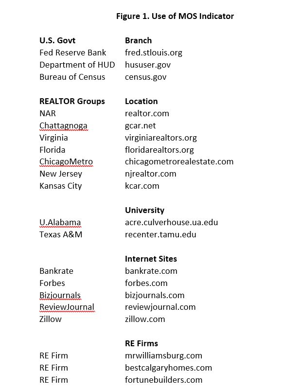
The value of the MOS indicator in Figure 1 is seen in its widespread use primarily in the housing sector driven by the U.S. Bureau of the Census surveys and reprinted by the U.S. Federal Reserve Banks (7). The Census publishes periodic reports on this indicator for New House Construction, Existing Houses, and New Multifamily. The National Association of Realtors circulates its periodic MOS indicator using sales and listings of houses through local Multi-List data. A wide range of local and state REALTOR organizations issue statistical reports which typically include monthly MOS estimates to identify market trends. The U.S. Department of Housing and Urban Development (8) includes a MOS estimate in its national housing reports. (8)  Further, frequent reports and references are available from local real estate firms, magazines and statistical reporting firms. In sum, a frequent evaluation of the demand and supply trends in housing and the impact on future transaction prices appears to be a valuable part of a housing market analysis.

All participants in real estate markets want a market analysis that provides an accurate assessment of potentially changing real estate prices from fluctuations in consumer demand and industry supply. Indicators such as those discussed in this paper contribute to a risk analysis of a future economic recession from possible loan defaults and the resulting impact on financial markets.

2. Data Needed

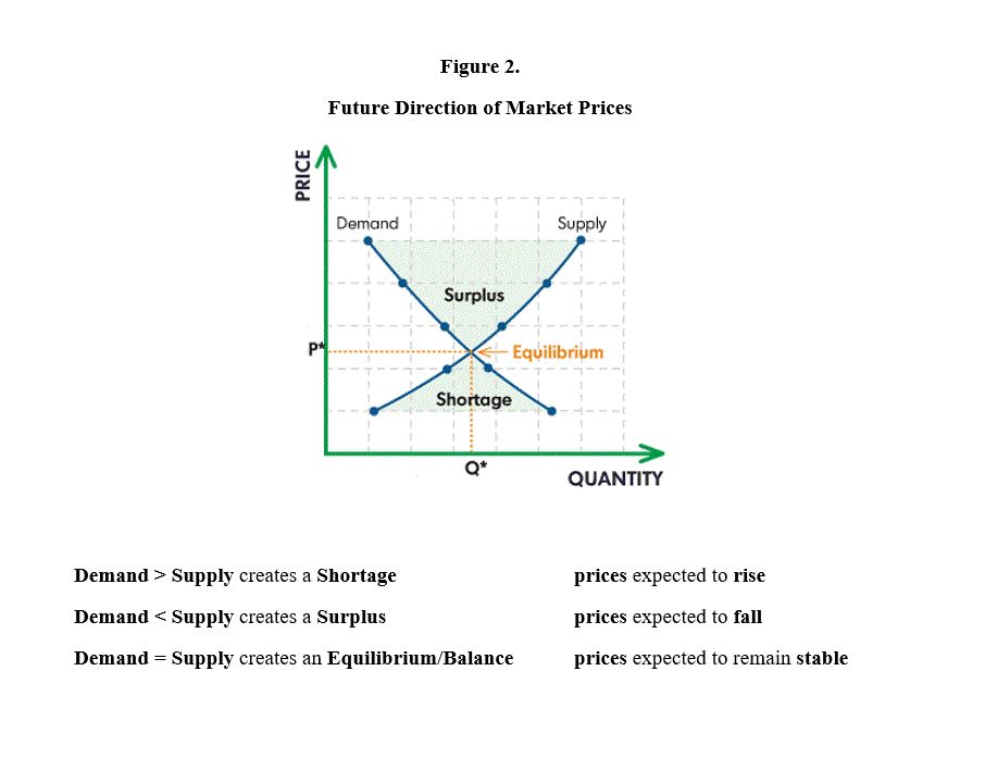
Buyers’ demand for the property is the average of the closed sales for the current period plus the previous 11 periods. The level of supply is represented by the active listing inventory available for sale. Combining the two allows the analyst to estimate whether the market is experiencing a shortage (demand > supply), surplus (demand < supply), or is in balance (demand = supply). These conclusions provide the needed insight to the analyst and the client on the overall trend and direction of future price.

The analysis of buyer demand and the level of supply are two independent calculations that track two different sectors of the market. Demand originates through overall and industry employment, income, savings, price expectations, and population characteristics. In contrast, supply markets rely on all construction costs, supply chain availability, skilled labor and wages, and land regulation. Both give signals such as current prices and costs to other parts of the real estate industry and profession (9).

A MOS indicator that reveals a current shortage (D>S) creates an incentive for potential buyers to offer a higher price in a competitive market with fewer contract restrictions. Concurrently, potential owners see higher prices causing higher capital gains and feel an incentive to bring additional properties to the market for sale. The result of the shortage is that both consumers and suppliers have incentives to react which causes a higher market transaction price.

When a surplus occurs, both buyers and sellers have reacted in opposite directions causing buyers to offer lower prices, potential sellers hold properties off the market, and the market transaction price drops. This article calculates both separately and combines them in three calculations to provide an opportunity to examine each in additional detail as needed.

3. Calculation of MOS

The MOS indicator is calculated by,

MOS = Supply  /  Demand ,

or,         active listings in the current month / avg. of closed sales in the current+ past 11 mos.

Analysts may prefer to be more inclusive by the inclusion of additional selected data and transactions. Examples include,

Listings:         Add condominiums and new construction in the current month

Sales:              Use condominiums and new construction in the current month

Use the median rather than the average because the median is not influenced by extreme values

Use the popular time period for closed sales which is (sales in the current month + sales in the previous 11 months) or select 3, 4, 5, and 6 months to better represent the local market

Add a “pending closing or sale”  representing an offer that has been accepted by the owners

Eliminate special monthly trends such as a change in seasonal sales or listings in winter, spring, or summer months.

Price Range:         Calculate a MOS for a price range to examine price trends for a specific group of properties in comparison to a MOS for the whole area.

When the demand and supply numbers are compared, the result provides a number of months to clear the properties available for sale indicating a soft or strong market. A shortage or surplus can be calculated, and statements can be made about expected future price changes seen in Exhibit 2. Thus, answering one question on current market conditions provides a number of useful results.

Closed sales, active listings, and the monthly MOS  for a larger metro area were available from a local MLS and university are shown in Figure 3  The MOS included historical sales is shown in column d with a 12-month average of sales including the current month and the prior 11 months, which equals 3409.1. The MOS for January Year 2, uses active listings in column b, 1305,  divided by 3409.1, or 0.38. The result is a shortage as demand is greater than supply. The rate of sales over the past 12 months requires 11-12 days to sell the existing listings (30 days x .38 = 11.4).

 

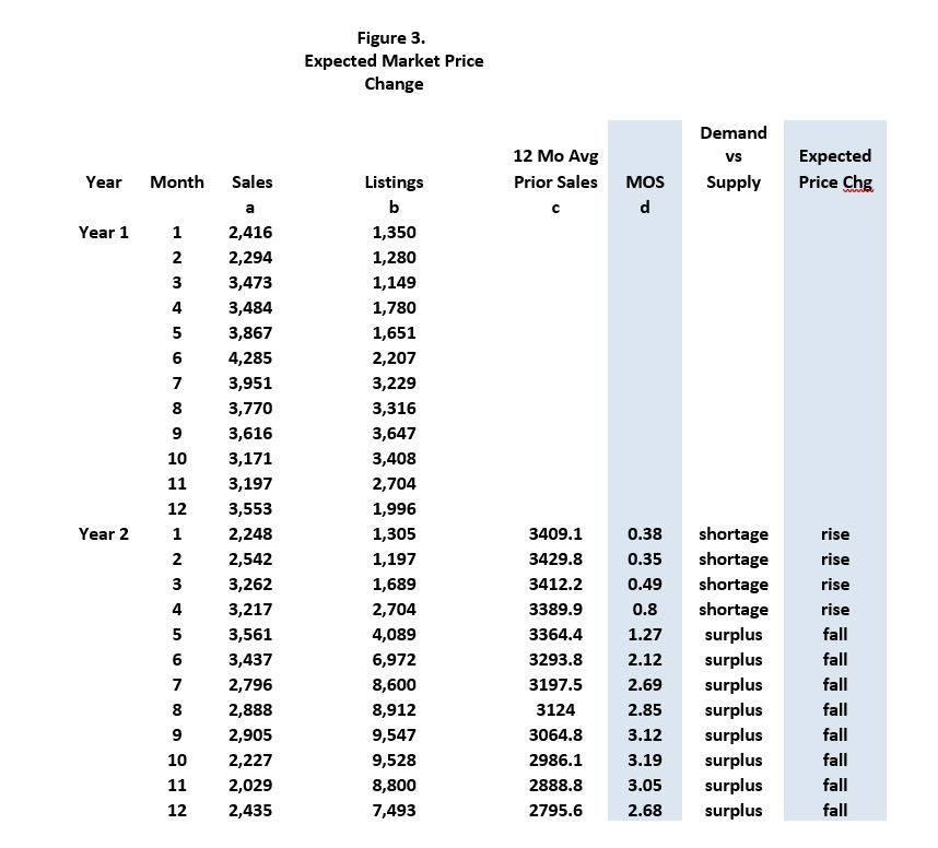
In Year 1, sales are larger than listings in 8 months. In Year 2, in the last 8 months of Year 2, Listings are greater than sales in the last 8 months. Market prices in Year 2 are expected to rise in the first four months from a shortage and fall in the remaining months of Year 2 from a surplus

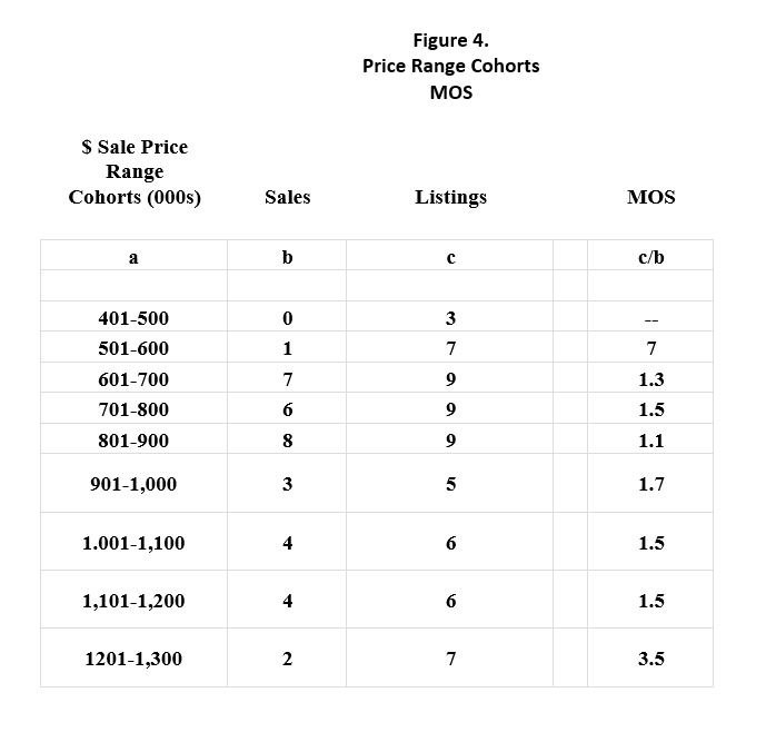
Price/range cohorts in Figure 4 are useful to determine if any specific cohort is not consistent with the overall market shown in Figure 3. Houses selling from $150,000 -$250,000 require about 2 months to sell and represent 5 percent of the total market. The rest of the properties in the table require around 3 months to sell. Properties within $300,000-$750,000 are 76 percent of this market and take 2.9-3.9 months to sell. The MOS numbers provide good support for the numbers in Figure 3.

4. Conclusions and Recommendations

A future market analysis can be expected to contain a thorough examination of price trends driven by underlying movements in the buyer demand for housing and is interaction with the available supply from owners.  Housing analysts will be asked to uncover data-driven market trends that will emphasize an increased level of statistical expertise, education, and experience in market analysis. This article contains a discussion and illustration of one important indicator that incorporates both residential demand and supply. Understanding how it is constructed and interpreted adds to the analyst’s toolkit and expertise.

This article arms the analyst on one readily available market indicator labeled the “months of supply” (MOS) which currently exists from a number of sources in a number of real estate markets, private companies, federal government, and academia. Further, this article shows how to calculate this statistic on data with figures available from a local Multiple Listing Service private data service, government, and university. The results provide a very valuable tool which combines a local estimate of buyer demand, a separate estimate of seller supply, and a future estimate of movement in sales prices. The conclusion should provide additional education and tools that the analyst can use to provide an additional level of accuracy in the estimate of future movement in market prices.

---

Endnotes

1. Federal National Mortgage Association, Announcement 08-30 Appraisal Related Policy Changes and Clarifications (November 14, 2008) page 3; Appraisal and Property Report Policies and Forms, Frequently Asked Questions) updated March 2009, page 2.: see also Selling Guide, March 01, 2013, B4-1.3-07, Sales Comparison Approach Section on Appraisal.
2. National Association of Realtors, Housing Forecast: Months Supply, (2023), www.realtor.com:“How Do You Calculate Absorption Rate” The Realtor.com Team, (November 30, 2015), 3 pages.
3. Texas A and M University Real Estate Center (TAMU), Housing Report for (City), monthly, www.recenter.tamu.edu
4. U.S. Census, Survey of Market Absorption of New Multifamily Units (SOMA),             www.census.gov
5. Appraisal Institute, The Appraisal of Real Estate, 15^th Edition, Valuation Process, chapter          4 Figure 4.1 Components of the Valuation Process, (2020), p.31, Chicago, Ill, chapters     15, 16.
6. Appraisal Foundation, Uniform Standards of Professional Appraisal Standards,       Standards Rule 1-3, Market Analysis and Highest and Best Use, (2024),  p.20, Washington
7. St. Louis Federal Reserve Bank, “Months Supply of New Homes,” latest edition,            https://fred.stlouisfed.org/series/MSACSR;  “Months Supply of Existing Homes,” latest          edition, https://fred.stlouisfed.org/series/HOSSUPUSM673N
8. U.S. Department of Housing and Urban Development “Appraisal Reporting             Requirements in Declining Markets,” Mortgagee Letter 2009-09, (March 2009), pages 2-           3
9. Samuelson, Paul, Economics, Supply and Demand, Bare Elements, Chapter 4, McGraw-        Hill, (1970),  55-72.