The Impact of Submarket Trends on Property Performance

I. Introduction

Location matters for how commercial real estate will perform over time. This statement will seem painfully obvious to industry practitioners, who may argue that (aside from timing and luck) location is the only thing that matters. However, in an age where capital flows across national borders relatively easily; when physical locations seem “optional” for a mobile workforce connected by the internet — does location still matter? And by how much?

In this article we investigate just how much location-specific factors influence commercial real estate performance, if at all. First, we update the results of Taylor, Rubin and Lynford (2000)[1] using panel data from specific commercial properties obtained from Reis, a provider of commercial real estate data that has been tracking building fundamentals like rents and occupancies since 1980. With quarterly data available from 1999, we now have seventeen years of time series covering two business cycles (expansion from 1999 to 2000; contraction from 2000-2001; expansion from 2002 to 2008; the 18 month recession from 2008-2009, and the recovery period from mid-2009 to the present). Not surprisingly, we find that location does matter when it comes to performance as measured by either property-level rent or revenue growth — consistent with prior literature (Capozza and Helseley, 1990).[2] However, we find that location matters even more during downturns, with submarket-specific factors accounting for up to two-thirds of how a building will perform during the recession of 2008-2009.

In the second part of the article we investigate whether location matters as much for “global cities” — cities perceived to be more connected to global investment flows and a mobile workforce. Somewhat counterintuitively, submarkets — the proximate neighborhoods where specific properties are located — matter even more for global cities, suggesting that cross-border capital flow and a mobile workforce actually magnify the importance of location instead of diminishing it.

II. Theory and Data

In frictionless environments with perfect and complete information, location should not matter for pricing and fundamentals. The supply of properties will instantaneously rise where demand is great, and ebb where demand falls; rents and vacancies follow accordingly, and equalize across locations. However, real estate is a lumpy, indivisible asset: it takes time for supply to be built and inventory does not adjust quickly even as rents fall, unless demand contracts so severely that properties are demolished, converted or left fallow. Tenants do not move across buildings seamlessly and lease structures stabilize income trends and affect decisions on how to set rent levels. There are location-specific factors that affect the desirability of specific geographies, so much so that most cross-MSA regressions using U.S. data usually need to exclude New York and San Francisco to determine whether the effects being investigated are systematic or are driven only by these “superstar cities.”
But how much does location influence the performance of a specific property? Taylor, Rubin and Lynford (2000)[3] measured this by estimating equations of the form:

pij=αMij+βSij+γbij+εij (1)

Where p represents measures of property-level performance for a specific building located in place i during time j, either in terms of revenue or rent growth. M represents metro-level measures of revenue or rent growth, and S represents submarket-level measures of revenue or rent growth. b is a vector of building-level attributes like age, size (in units or square feet of space, depending on the property type), or number of floors, that plausibly drives property-level performance. ε is the error term, assumed to be independent and identically distributed. α, β, and γ are the estimated coefficients for the respective independent variables. The key question they were  trying to answer was whether market practitioners ought to use market/metro/MSA-level variables, which had the advantage of being more readily available (estimates for rents and occupancies are produced occasionally by the U.S. Census via various surveys), or if using more disaggregated submarket-level variables offered an advantage. From cross-sectional estimates available at the time, the authors concluded that submarket-level variables accounted for between forty to fifty percent of a property’s overall performance, while only approximately ten percent was explained by metropolitan market factors.

We now have the advantage of seventeen years of quarterly data from 1999 to 2015, allowing for analysis over time. Geographical definitions of submarkets remain based on patterns of locational preference expressed by end-users (tenants or owners) of specific property types, accounting for vehicular and mass transportation patterns, and the location of competitive projects.

The advantage of such an approach to geography is specifically what we are investigating in this article: does granularity matter? Or should we simply use larger metro-level aggregations in our analysis of property-level performance?

III. Analytical Approach

The specification from equation (1) regresses building-specific revenue levels on contemporaneous and the first three lags of metro-level revenue levels; contemporaneous and the first three lags of submarket revenues; the first two lags of property-level revenue; and fixed property characteristics for the office, apartment and retail properties in our database. This matches the methodology of Taylor, Rubin and Lynford, but given the availability of a larger panel property-level data over a longer time series, we can exploit new angles.

III.A. Segregating Across Time

Since revenue growth and rent trajectories are subject to business cycles, we segregate the analysis of how much location-specific drivers affect property-level performance by time period. Specifically, we run six separate regression analyses, covering economic booms and subsequent recessions:

1. From 1999 to around the end of 2000, which captures the tech boom.
2. From 2000 to around 2001 to 2003. The reason for the dispersion around the end point has to do with sector-specific troughs: for most apartment submarkets, recovery for both occupancies and rents commences sooner than for office properties, within the same MSA. This is also metro- and submarket-specific: we adjust the time when the “tech bust ended” depending on when rent growth turned positive — however sluggish.
3. From 2003 to 2004 to anywhere from early to late-2008. This captures the housing boom, when economic growth lifted most sectors, including commercial real estate. Again, the beginning and end points are determined by when submarket fundamentals “turned,” specific to each property type. In hindsight, for example, retail was the canary in the coal mine, with absorption that turned negative in early 2008, well before the crash of Lehman Brothers shifted the Great Recession into high gear. Office properties, on the other hand, did not really experience a large pullback in rents until the start of 2009.
4. From mid- to late-2008 to around 2009 or 2010. This period captures the last recession, which was the most severe contraction in economic activity that the U.S. experienced since the end of World War II. Around 8.4 million jobs were lost and the recession lasted for 18 months, officially ending in June 2009. But national apartment vacancies continued rising to record highs until the end of 2009; office vacancies did not peak until the end of 2010, and shopping center vacancies continued rising until the third quarter of 2011, even though rent growth had already turned mildly positive about a year prior.
5. From 2010 to 2011 to the end of 2015. This captures the ongoing recovery period, characterized by slow GDP growth of approximately 2 percent per year, low interest rates that ended up boosting property values for a select group of buildings that transacted and extreme variability in recovery rates for commercial property, with multifamily recovering very quickly and office and retail continuing to limp along.

A sixth regression is conducted across the entire period from 1999 to 2015 to calculate the overall effect of submarket and metro-level variables on property-level performance.

III.B. Segregating Across Space

The complete panel of property-level performance information[4] is aggregated up, weighted by either units (multifamily) or square feet of rentable space (office and retail), to form submarket and metro-level trends. One additional complication that we considered in this article is the endogeneity[5] of property-level performance and submarket and metro-level trends — papers that simply regress property-level performance on the LHS and submarket and metro-level trends on the RHS are biased towards a positive result — since each property’s performance helps determine what submarket and metro-level aggregated trends look like.

To sidestep this circularity, we recalculate submarket- and metro-level trends excluding each property being studied. This renders the aggregated trend calculation to be slightly different from Reis’ published figures, particularly when we are examining the case of a large property that influences a relatively small submarket delineation’s performance aggregates. This also required significant computing power, since separate regressions needed to be conducted for each subject property relative to submarket-ex-subject and metro-ex-subject. A statistical loop program was written in Stata to run the calculations and summarize the results. Fixed property-specific characteristics like the building’s age, size, total units, unit mix in a specific apartment building, and number of floors for office buildings, were included in the regression to represent property-level drivers of revenue.

Combined with the six time-specific regressions outlined in the preceding section, this approach carefully addresses the central question of, “By how much do submarket-specific drivers affect or determine property-level performance?”

IV. Results

The regression framework allows us to estimate the marginal effects of market-level, submarket-level, and property-level drivers of revenue, including lagged variables rendering the analysis subject to autocorrelation, but assuming that rent and revenue levels in commercial real estate are not correlated over time is equally incorrect. In any case, Durbin Watson statistics appear reasonable and the results quantify the relative weight of metro, submarket and structural property factors in determining property revenue levels.

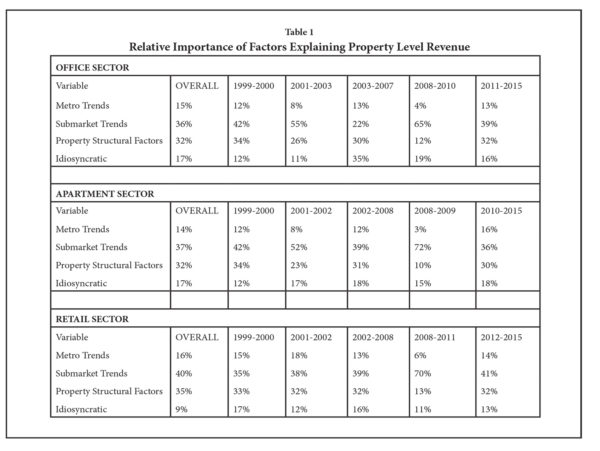
The results are presented in Table 1 below. Considering the entire time frame from 1999 to 2015 yields a breakdown similar to the Taylor, Rubin and Lynford paper from 2000, with anywhere from 36 to 40 percent of all property revenue variance explained by submarket trends. Property structural characteristics explain an additional 32 to 35 percent, and anywhere from 9 to 17 percent of the variance is left unexplained by the model, relegated to the error term and considered idiosyncratic.[6]

Submarkets Matter, but Particularly So During Downturns
Partitioning the analysis into discrete time periods that represent economic booms as well as downturns is particularly revealing. Consider the office sector. During the tech boom the proportion of property level revenue explained by submarket trends rose from the “overall” figure of 36 percent encompassing the entire time period to 42 percent: a visually appealing but statistically insignificant difference. But when the tech bubble burst, submarket trends came to dominate the story, accounting for 55 percent of property level declines in revenue. The same pattern was observed during the even more severe downturn from 2008 to 2009. The recession began on December 2007 and ended in June 2009, but national office vacancies did not reach their peak until the third quarter of 2010. During this time, 65 percent of property level performance was determined by submarket drivers. Multifamily and retail properties exhibit similar patterns, with the proportion of property level revenues explained by submarket trends rising to 70 to 72 percent during the Great Recession. The most recent period of recovery, which commenced at different points in time depending on the property type (2010 for apartments, 2011 for office, 2012 for retail), exhibited figures that generally resemble the results for the overall time frame, with submarket trends accounting for 35 to 39 percent of property level revenue variation.

Why might submarket drivers matter more during downturns? There is a large body of literature on shocks, contagion and how asset prices and other measures of performance tend to converge during downturns, as market participants stampede out of risky assets and seek safe havens like U.S. Treasuries.[7] Commercial real estate is apparently not immune to such effects. During the tech bust, Reis data shows that fully leased office buildings located in San Francisco submarkets that suffered from the closure of dot com companies lowered rents by almost as much as neighboring properties in submarkets not dominated by a cluster of tech-related tenants whose vacancy rates shot up.

From these results it seems clear that market-level data is too coarse to use as a proxy for how a property will perform. Where available, analysts should use more disaggregated data like submarket trends when explaining or predicting the performance of a single building or a small group of properties.

V. But Do Submarkets Matter for High-Performing “Global” Cities?

Whether the term is “global,” “superstar,” “24-Hour” or “18-Hour” cities, there are a handful of places that stand out because of the way they attract investment, households, and generate employment and output. Hugh F. Kelly (2016)[8] identifies New York, Miami, San Francisco, Washington, D.C., Boston and Chicago as part of this cluster of high-performing cities where vibrant economic activity goes hand in hand with strong property price performance. Would submarkets matter less for a place like New York City, if the rising tide of metro prosperity lifts all boats?

To address this, we segregate the analysis using an indicator variable to separate the effect of being in the “24-Hour city” group above. If submarkets matter less, the relative effects presented in Table 1 should decline for “submarket trends.” An interesting trend emerges.

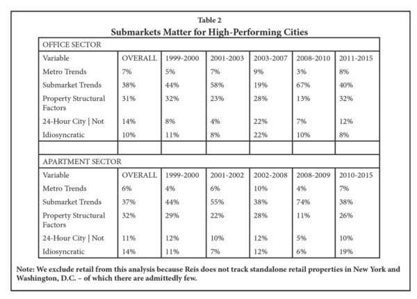
Separating the analysis across high-performing cities does not diminish the importance of submarket factors in determining property performance. Submarket trends retain their significant impact, particularly during downturns. The explanatory power of metro-level trends did decline, but it is likely that designations of being a high-performing “global” city is correlated with metro trends, reducing the latter’s impact.

It is perhaps not so surprising that what drives high performance cities are high performance neighborhoods. During downturns, the resilience of specific neighborhoods and submarkets in these high performance cities really help bolster the performance of properties located within. Consider how properties in the Queens submarket of New York City performed in the last downturn. New York was arguably the epicenter of the financial services meltdown of late 2008 that lasted through 2009 — but apartment properties in the Queens submarket actually had asking and effective rents rise, on average, by 1.4 percent and 1.2 percent, respectively. Regardless of whether vacancies were on the high or low side of the submarket average of 2.1 percent, a large majority of properties in Queens were able to raise rents during a time of major upheaval — because the submarket itself was benefiting from an exodus of households from more expensive parts of Manhattan;[9] households that could no longer afford premium rents but who still wanted to live within the five borough area, within walking distance of New York City’s famed subway system.

VI. Summary and Future Research

Location therefore does seem to matter for property performance — which is in line with the intuition of market participants and investment managers. Even in the age of 24-hour cities benefiting from global capital flow and a mobile, connected workforce, submarkets still matter.

This suggests that the use of granular data is superior to more aggregated trends. But this begs the question of whether tracking the performance of a narrowly defined group of comparable properties is even better than using submarket data when it comes to explaining and predicting the performance of a single building. Theoretically this seems to make sense, and much effort is expended by industry analysts defining their “comp group” appropriately, against which they benchmark the performance of their subject property.

The argument against going “too granular” for forecasting purposes is that one may encounter higher levels of idiosyncratic variability that submarket aggregations will tend to smooth out; if a comp group of ten is better than using the entire submarket, it does not follow that a comp group of one is superior.

But would submarkets matter as much if you were the marquee property in the neighborhood? Consider a small submarket with a single, large multitenant office property housing a major employer located right in the center; a set of smaller buildings surrounds the large property, forming the submarket. During downturns, the large office building may in fact withstand submarket trends better than the smaller properties. Conversely, suppose the large office building loses its anchor tenant during relatively calm economic times, forcing it to lower rents significantly. This is presumably one case when a rather large tail will wag the entire dog, compelling the smaller properties to lower rents as well even without the pressure of a recession. We control for this somewhat by our exclusion procedure outlined in Section III.B, but further study appears warranted.

Future research papers will investigate these questions.

---

Endnotes

1. Taylor, M., Rubin, G., and Lynford, L. Submarkets Matter! Applying Market Information to Asset-Specific Decisions. Real Estate Finance, Fall 2000, pp. 7-26.
2. Capozza, D. and Helsley, B. The Stochastic City. Journal of Urban Economics, 28(1990), pp. 187-203.
3. Supra
4. On an ongoing basis, Reis surveys and receives data downloads from building owners, leasing agents and managers which include key building performance statistics including, among others: Occupancy rates; rents; rent discounts and other concessions; tenant improvement allowances; lease terms; and operating expenses.
5. Endogeneity in regression analysis refers to a situation where the predicted variable affects independent variables; the “left hand side” affects the “right hand side” so the explanatory variables are not really independent.
6. Idiosyncratic in this context refers to what remains unexplained by the overall analytical framework.
7. For a classic summary, refer to Charles Kindleberger’s Manias, Panics and Crashes: A History of Financial Crises.
8. Kelly, Hugh F. 24-Hour Cities: Real investment performance, not just promises. Routledge, New York: April 2016.
9. For comparison, effective rents fell by anywhere from 1.1 percent (Bronx County) to 11.3 percent (Upper West Side) for other New York City submarkets. The amount of decline in effective rents appears correlated to relative rent levels, with more expensive neighborhoods taking a bigger hit. Kings County – Brooklyn – had effective rents decline by 3.3 percent, but the submarket had by that time become relatively expensive given the surge in property prices and rents in newly gentrified areas like the DUMBO neighborhood.